This is an adapted, abbreviated, edited version of the original version of Par Martin Grandjean's "Introduction to Network Visualization with GEPHI" (2013), published under a CC BY 3.0 CH license. Some instructions and screenshots have been revised because of changed interface features in the newer version of Gephi (v. 0.9.1).
This revised version of Grandjean's tutorial was created by Alan Liu in February 2016 for the purposes of a beginning workshop on digital humanities methods. Note: Grandjean has since published a new version of his tutorial (2015). For the purposes of his workshop, however, Liu chose the original tutorial to adapt because its data set (nodes and edges .csv files) is simpler for the beginner to grasp conceptually. Also, the later tutorial requires additional Gephi plugins to work with geolocation, some of which at in Feb. 2016 were not available for the new 0.9.1 version of Gephi.
1. Short introduction to Social Network Analysis
A network consists of two components : a list of the actors composing the network, and a list of the relations (the interactions between actors). As part of a mathematical object, actors will then be called vertices (nodes, in Gephi), and relations will be denoted as tiles (edges, in Gephi).
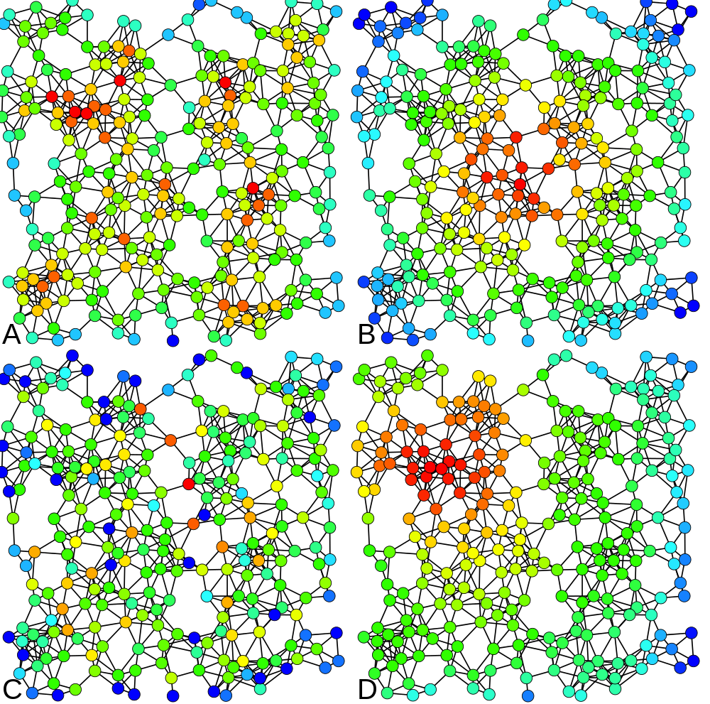
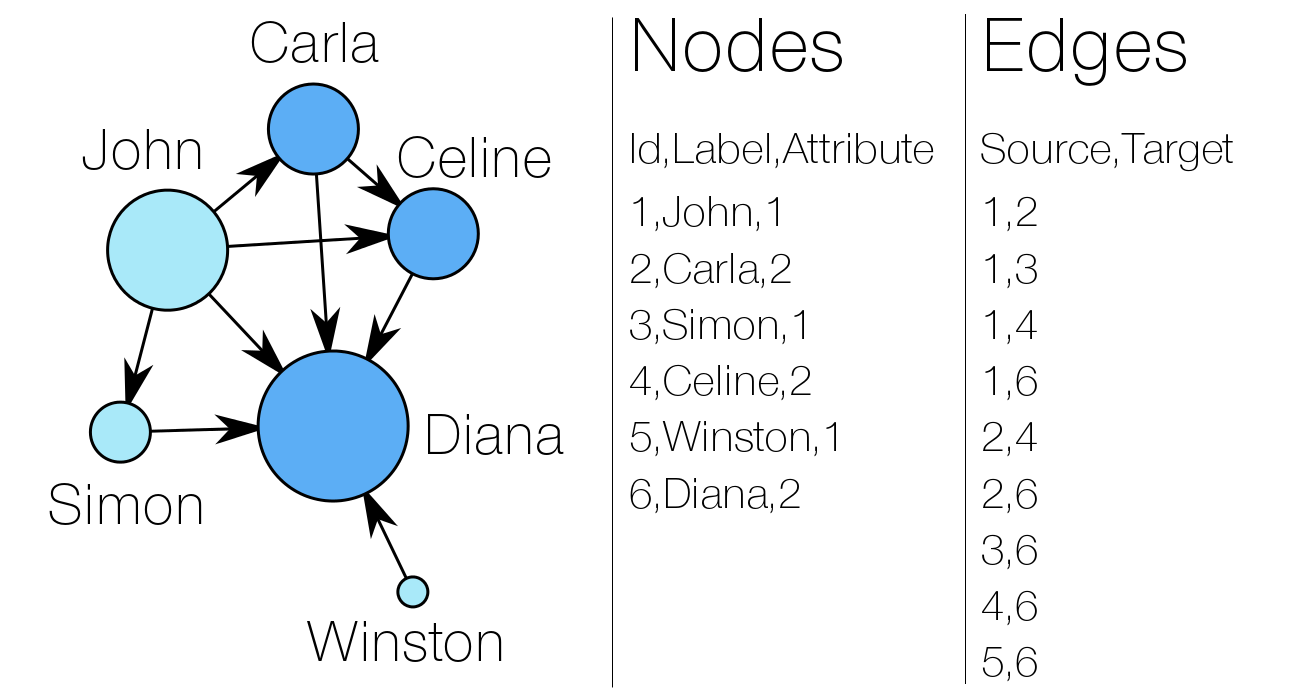
At the left, you can observe a very simple social graph, with both lists made explicit. Two attributes are attached to the nodes : a label (his or her “name”) and a numeric attribute (akin to the sex of people here, for example). In the edge list, “Source” and “Target” entries refer to the nodes’ numeric identifiers (Id). In our example, the “sex” attribute determines the color of the nodes. The size of a node depends on the value of its “degree centrality” (its number of connexions). The centrality measures are essential metrics to analyze the position of an actor in a network. They come in many variations, as shown at right (A = Degree centrality, number of connexions ; B = Closeness centrality, closeness to the entire network ; C = Betweenness centrality, bridges nodes ; D = Eigenvector centrality, connexion to well-connected nodes).
(Claudio Rocchini, Wikimedia)
3. Downloading the data set for this tutorial
Download both the following CSV files. Be sure to save them with a .csv file extension. (If you need to, you can paste their contents into a plain-text file with a .txt extension, then rename the file with a .csv extension).
Note: "CSV" (standing for "comma separated values") refers to a family of plain-text format data files in which the values are separated by a a comma, semi-colon, tab, or some other separator. Grandjean's csv files use a semi-colon separator. CSV files are a common way to store data sets because they can be easily migrated into other formats. For example, one can open them in Excel as a spreadsheet (and one can save spreadsheets in CSV format).
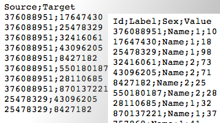 The data consist of a random selection of Twitter users and their “followings” relations. The “Nodes” file contains the identifiers of each nodes, their label, a sex attribute and a random value that will be usefull to play with visualization tools hereafter. The “Edges” file contains a list of identifiers couples showing who follows who.
4. Importing the data into GEPHI
![]()
![]()
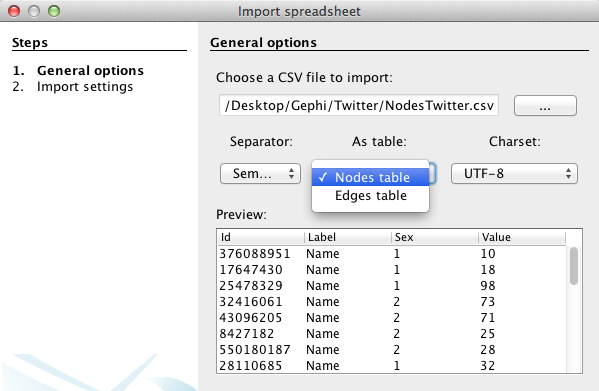
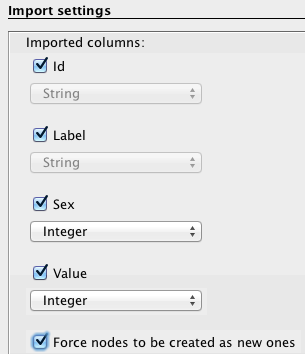
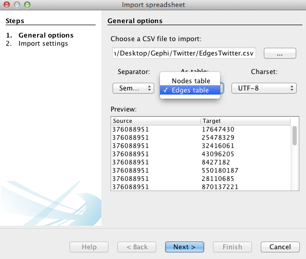
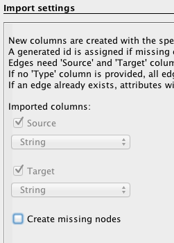
Start Gephi on your computer and create a “new project” in the start menu. In the Data Laboratory, click on “Import Spreadsheet” to open the import window and import your “nodes” file.

5. Visualization!
The action now takes place on the overview panel (chosen through the tab below).
![]()
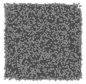
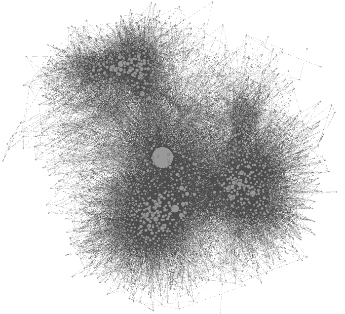
Clicking "overview" produces an overview of the graph spatialized randomly that is completely unreadable (below).
To make the graph readable, we will adjust node sizes, apply a spatialization layout algorithm (to separate out nodes into meaningful clusters), and then use colors and labeling to make attributes visible:
Adjust Node Sizes

- In the "Appearance" panel at left of the Gephi workspace, select "Nodes" (#1 in example diagram).
- With the "Unique" tab selected under "Nodes," click the icon indicating size adjustment (#2), and adjust as you wish.
- You can also select the "Attributes" tab (in newer versions of Gephi, "Ranking" tab) and experiment with settings. For example,you can click on the “Spline” blue link (#4) if you wish to edit the shape of the spline. You can use one of the pre-set templates in the spline choices if you wish. (An explanation of "spline") (Be aware that linearly double the radius of the nodes is more than double the area because of the power function).
Spatialization (Layout in Space)
 Spatial visualization is the biggest part of what you can do in Gephi! While it is possible to play (and lose yourself) with various visualization capabilities, I propose a method appropriate to the data set for this tuturial.
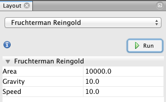
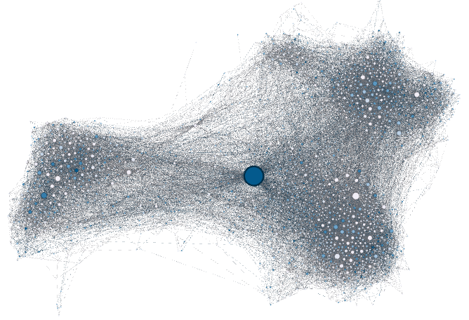
In the "Layout" panel at the left of the Gephi workspace, start by choosing the Fruchterman Reingold layout algorithm, use the same values as in this model (10000 10; 10). Then click on "Run" and let Gephi begin adjusting the position of the nodes. (This visualization distributes nodes according to a physical metaphor of attraction-repulsion, as if the nodes were magnets). You’re already able to distinguish communities (more densely connected parts of the network). Let the function run until the graph is stabilized. You can scroll your mouse to zoom in and out of the graph. Then you can use the little blue magnifying glass (at the bottom left of the frame of the central graph panel in the Gephi workspace) to re-center the graph.
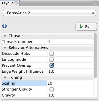
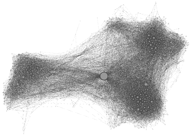 Then, in a second stage of spatialization, use the Force Atlas 2 layout algorithm to disperse groups of nodes further, providing more space around larger nodes. (Be careful, the parameters you enter can significantly alter the final appearance.) In the parameter options for the Force Atlas 2 layout, check “prevent overlap” and change “Scaling” to 10). Then click on "Run." Let the function run until the graph is mostly stabilized.
Set Node Colors

- In the "Appearance" panel at the left of the Gephi workspace (with "Nodes" still selected), click on the icon for setting colors (#1 in diagram at left).
- Then click on "Attribute." Because the nodes in this tutorial data set have attributes (gender), you can color them regarding their “sex” attribute (denoted by a value of 1 or 2 in the csv file) or simply with their degree centrality.
- To color by attribute, click on the drop down menu (#3 in diagram) and choose the attribute you wish to differentiate by color.
Label the Nodes
 To display labels for the nodes based on their attributes, do the following:
- At the bottom right of the graph display in the Gephi workspace, click on the icon for "label text settings" (#1 in diagram at left).
- A little panel will open up on which you can choose the attribute(s) you wish to see displayed as labels, e.g., "sex" (#2 in diagram).
- Then click on the "T" icon at the lower left of the frame of the graph panel (#3) to display the labels. In the example at left, for instance, sex is labeled as "1" or "2" (the numerical values assigned respectively to mals and females in the data set nodes.csv file).
- If you wish to have more control over the formatting and other features of the labels, click on the icon at the lower right of the frame of the graph panel (#4) to open up a panel for label details.
Adjust Final Details

To adjust the final look of your Gephi graph:
- Click on “Preview” to change to the preview mode (#1 in diagram at left).
- Then click on "Refresh" (#2 in diagram). .or trimming the final details.
- Adjust settings as you wish. Unlike during previous stages, changing settings in this menu is reversible, and do not affect the structure of the graph. Be aware that due to its large size, the graph may take a few seconds to update after each change (click on “refresh” to apply changes).
- To export your final graph as a .svg, .pdf, or .png file, click on the Export icon at the lower left (# 3 in diagram).
6. Other features
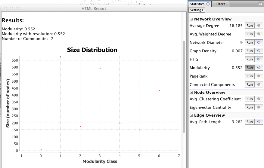 The visualization is only one step. Network analysis often requires other mathematical means to provide the researcher with a satisfactory result. Feel free to explore the “Statistics” menu (right), for example by playing with degree measures, density, path length, modularity.
A network contains internal subdivisions called communities. There are methods that permit to highlight these communities, which depend on the comparison of the densities of edges within a group, and from the group towards the rest of the network. More here!
In the right column of the “overview” page, click on Statistics/Modularity/Run to display the modularity window. Choose a resolution (between 0.1 and 2), click OK and close it.
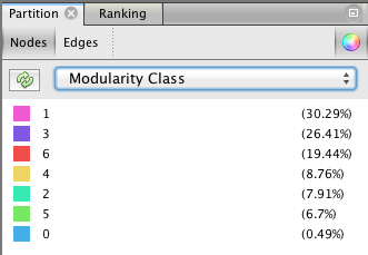
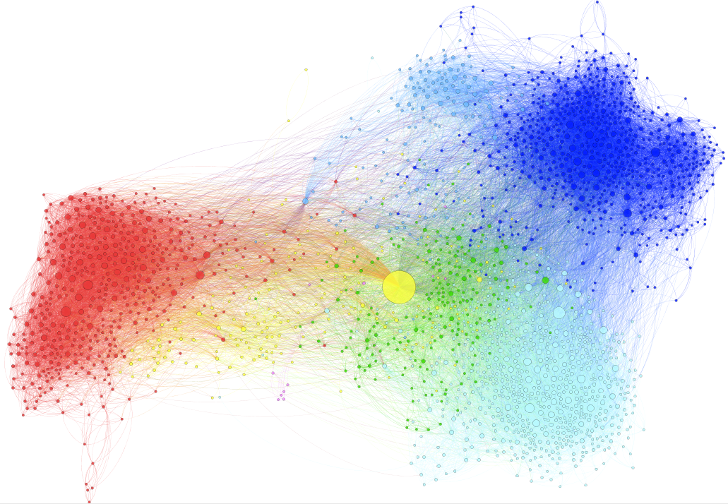 The next step takes place in the Partition menu situated in the left column. Select “Nodes” and “Modularity Class” (rolling menu). You will be then able to modify the colors attributed to the detected communities by clicking on them.
Do not hesitate to repeat this operation with many “Resolutions” ! If you decide to do so, you must deselect and reselect “Modularity Class” in the left column, and refresh color calculation.
Conclusion
Do not forget that what you see of GEPHI is just the tip of the iceberg because the application allows you to install very interesting plugins, has various tutorials and offers a very active forum.
I hope this tutorial has been a way to whet your curiosity to go further in social network analysis, and I am delighted to see your accomplishments!
[Go to Par Martin Grandjean's original version of this tutorial.]